Hey curious engineers, welcome to the tenth issue of the The Main Thread (first milestone for this newsletter).
In the last issue, we explored why tokenization matters, how it controls costs, shapes what models can learn, and encodes bias before training begins.
Today, we're going under the hood. How do tokenizers actually learn which fragments to create? Why does GPT use one algorithm while BERT uses another? And what makes these approaches so powerful that every major LLM depends on them?
Let's start with a problem.
The Impossible Trinity: Why Nothing Works Perfectly
Imagine we are designing a tokenizer from scratch. We have three requirements:
Universality: Handle any input without failure including misspellings, rare words, emoji, languages we have never seen.
Efficiency: Produce short sequences so attention is fast and context windows stretch further.
Robustness: Degrade gracefully on challenging inputs rather than breaking or losing information.
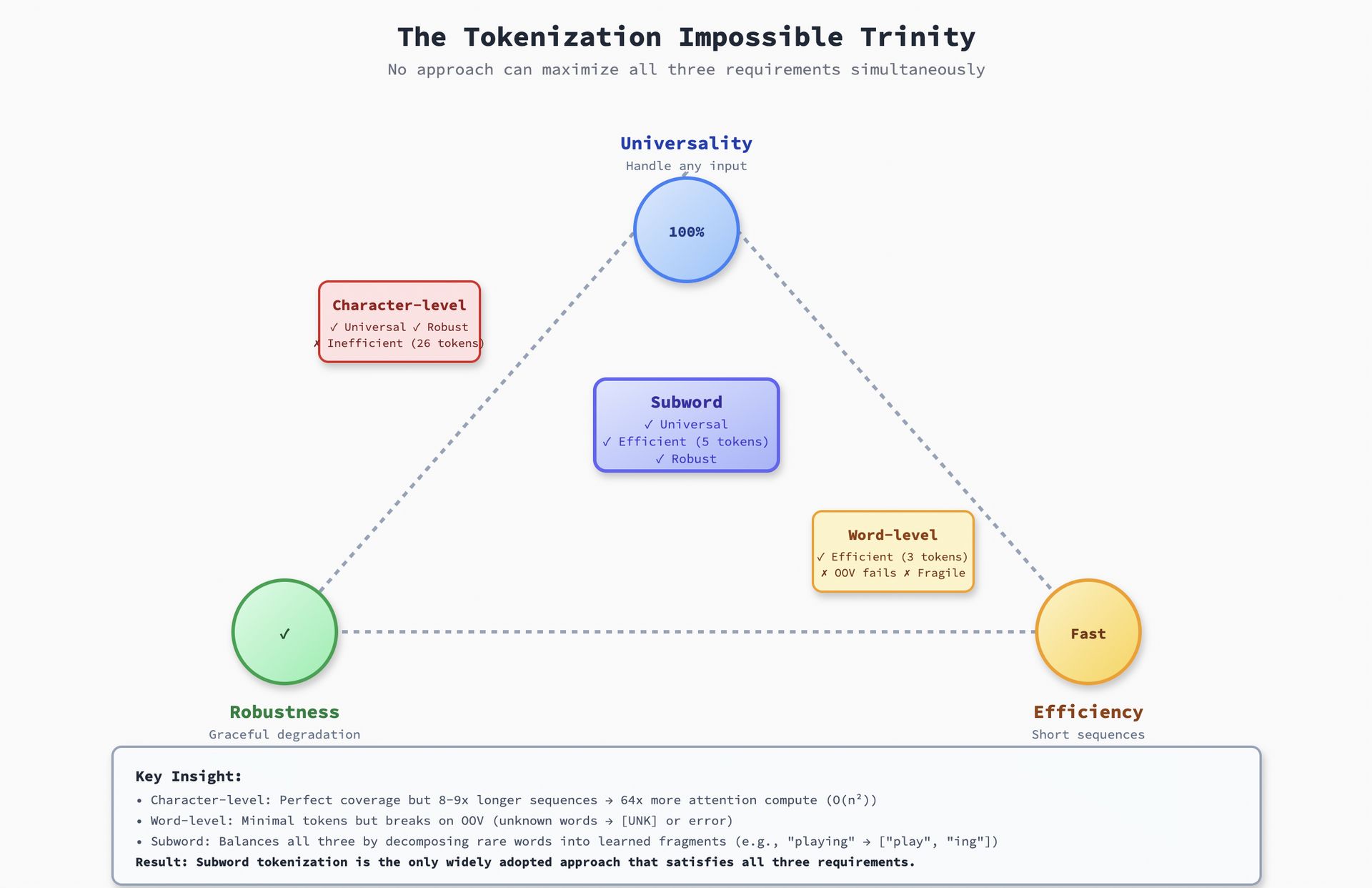
Here's the problem: we can't maximize all three simultaneously.
Character-level tokenization gives you perfect universality (every string is just characters) and robustness (misspellings don't break anything), but it's catastrophically inefficient. The word
"machine learning"becomes 18 tokens. Our context window fills up 8-9x faster, and attention becomes 64x more expensive(O(n²)).Word-level tokenization is maximally efficient—the word
"machine learning"becomes 2 tokens. But it fails on out-of-vocabulary (OOV) words. What if we encounter the word"supercalifragilisticexpialidocious"?Oour tokenizer outputs[UNK], and the model loses all information. Zero robustness.Subword tokenization finds the middle ground. Common words stay atomic. Rare words decompose into familiar fragments. Nothing becomes
[UNK]. We get universality + efficiency + robustness—not perfectly, but well enough for production.

The Impossible Trinity
This is why every modern LLM uses subword tokenization. GPT, BERT, T5, LLaMA, Claude—all of them. The question isn't whether to use subwords, but which algorithm to choose.
Let's explore the three that won.
Algorithm 1: BPE (Byte Pair Encoding)
This algorithm is primarily used by: GPT-2, GPT-3, GPT-4, RoBERTa, LLaMA, Mistral.
BPE is beautifully simple: repeatedly merge the most frequent pair of adjacent symbols.
How It Works
Start with a base vocabulary of individual characters (or bytes): ['a', 'b', 'c', ..., 'z', ' ', '.', ...]
Count all adjacent pairs in our corpus
Find the most frequent pair (e.g., 'e' + 's' appears 12,847 times)
Merge it into a new token ('es')
Repeat for N iterations (typically 30K-50K merges)
Let's watch BPE tokenize the word "newest":

BPE Merge Iterations on “newest“
👉 Initial state: ['n', 'e', 'w', 'e', 's', 't'] → (6 tokens)
👉 After learning "es" merge: ['n', 'e', 'w', 'es', 't'] → (5 tokens)
👉 After learning "est" merge: ['n', 'e', 'w', 'est'] → (4 tokens)
👉After learning "new" merge: ['new', 'est'] → (2 tokens)
Why This Works
BPE exploits Zipf's law: common patterns appear far more frequently than rare ones. By merging frequent pairs, we are building a compression codebook optimized for your training distribution.
This is essentially Huffman coding for text—short codes for frequent patterns, longer codes for rare patterns. Information-theoretically optimal (Shannon, 1948) if our deployment distribution matches our training distribution.
The Core Code (Simplified)
def train_bpe(corpus, num_merges):
  vocab = set(corpus)  # Start with characters
  merges = []

  for i in range(num_merges):
    # Count all adjacent pairs
    pair_counts = count_pairs(corpus)

    # Find most frequent pair
    best_pair = max(pair_counts, key=pair_counts.get)

    # Merge it everywhere in corpus
    corpus = merge_pair(corpus, best_pair)

    # Record this merge for encoding later
    merges.append(best_pair)
    vocab.add(''.join(best_pair))

  return vocab, merges
That's it. No neural networks, no gradients—just greedy frequency-based merging.
The Byte-Level Twist
GPT-2 introduced a critical innovation: byte-level BPE.
Instead of starting with Unicode characters, we start with UTF-8 bytes (0-255). Why?
Universal coverage: Every possible string is representable as bytes.
Fixed base vocabulary: 256 tokens, regardless of language or script.
No normalization hell:
"café"and"café"(NFC vs NFD) are handled identically.

Byte Level BPE Encoding
This is why GPT-3/GPT-4 handle emoji, code, and 100+ languages gracefully despite being trained primarily on English.
Algorithm 2: WordPiece
This algorithm is primarily used by: BERT, DistilBERT, ELECTRA.
WordPiece improves on BPE by asking: instead of merging the most frequent pair, what if we merge the pair that maximizes likelihood of the training data?
How It Differs from BPE?
BPE picks the pair with the highest raw count: if "es" appears 12,847 times, merge it.
WordPiece picks the pair that maximizes pointwise mutual information (PMI):

PMI Equation
High PMI means x and y appear together far more often than we'd expect if they were independent. This captures statistical dependency, not just frequency.
Why This Matters?
Consider two pairs:
"th"appears 50,000 times (very frequent)"qu"appears 5,000 times (less frequent)
BPE merges "th" first because it's more frequent.
But "qu" almost always appears together in English—high PMI. "th" is frequent but appears in many unrelated contexts—lower PMI.
WordPiece merges "qu" first because it's a stronger statistical unit.
The Result
WordPiece tends to produce vocabularies with more linguistically coherent fragments:
Morphemes:
["un", "ing", "ed", "tion"]Common bigrams with high dependency:
["qu", "ph", "ch"]
This is why BERT's tokenizer feels more "linguistic" than GPT-2's—it optimizes for statistical coherence, not just frequency.
The Core Code (Simplified)
def train_wordpiece(corpus, num_merges):
  vocab = set(corpus)
  for i in range(num_merges):
    pair_scores = {}
    for pair in all_pairs(corpus):
      # Score by PMI instead of raw frequency
      score = pmi(pair, corpus)
      pair_scores[pair] = score
      # Merge pair with highest PMI
      best_pair = max(pair_scores, key=pair_scores.get)
      corpus = merge_pair(corpus, best_pair)
      vocab.add(''.join(best_pair))
  return vocab
Note: The exact PMI formula used internally isn't publicly documented by Google, so implementations often approximate it with likelihood-based scoring.
Algorithm 3: Unigram LM
This algorithm is primarily used by: T5, mT5, ALBERT, XLNet
BPE and WordPiece are deterministic and greedy—they make local decisions (merge this pair right now) that can't be undone. Unigram LM takes a radically different approach: start with a large vocabulary and probabilistically prune it.
How It Works
Start with a huge vocabulary (e.g., 1M tokens from all possible substrings).
Assign each token a probability based on corpus frequency.
For each token, compute: "If I remove this token, how much does likelihood drop?"
Remove the 10-20% of tokens that hurt likelihood the least.
Re-estimate probabilities with EM algorithm.
Repeat until we reach target vocabulary size (e.g., 50K).
The Key Insight
Unlike BPE/WordPiece, Unigram LM is probabilistic. It doesn't produce a single deterministic tokenization—it outputs a distribution over possible tokenizations.
For "machine learning", it might give:
["machine", "learning"]- 70% probability["mach", "ine", "learning"]- 20% probability["machine", "learn", "ing"]- 10% probability
During training, we can sample from this distribution (subword regularization), which acts as data augmentation and improves robustness.

Unigram Forward Backward Algorithm
Why This Wins for Multilingual Models
T5 uses Unigram LM with SentencePiece, which adds another trick: train on sampled data with oversampling of underrepresented languages.
If our corpus is 60% English, 30% European languages, 10% everything else, SentencePiece can oversample that 10% during tokenizer training so they get fairer vocabulary allocation.
Result: mT5 handles 101 languages far more equitably than GPT-3.
The Core Code
def train_unigram(corpus, target_vocab_size):
  # Start with all possible substrings
  vocab = extract_all_substrings(corpus)

  while len(vocab) > target_vocab_size:
    # Estimate token probabilities with EM
    probs = estimate_probabilities(vocab, corpus)
    # For each token, measure loss if removed
    losses = []
    for token in vocab:
      loss = compute_likelihood_loss(corpus, vocab - {token})
      losses.append((token, loss))
      # Remove tokens with smallest loss impact
      tokens_to_remove = sorted(losses, key=lambda x: x[1])[:pruning_size]
      vocab -= {t for t, _ in tokens_to_remove}
 return vocab
This is far more computationally expensive than BPE (EM iterations over the full corpus), but it produces globally optimal vocabularies.
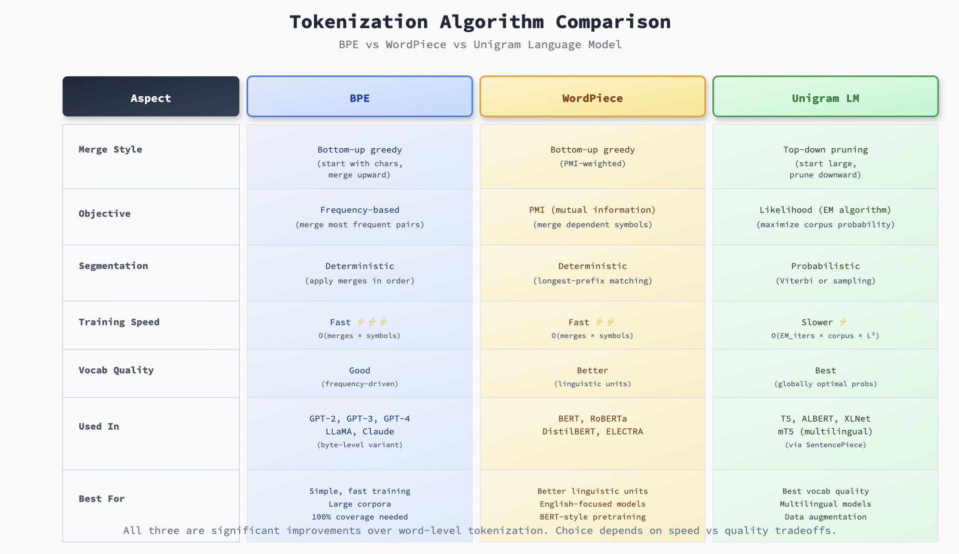
Side by Side: Which Algorithm When?

Tokenization Algorithm Comparison
The Deeper Pattern: Why Frequency-Based Learning Works
All three algorithms exploit the same fundamental insight: natural language has compressible structure.
Languages aren't random. We reuse common sounds, morphemes, and word parts rather than inventing completely new forms for every concept. This creates Zipfian distributions—a small number of units appear extremely frequently, while the long tail appears rarely.
This non-uniform distribution is exactly what compression algorithms exploit:
BPE builds a frequency-based codebook (like Huffman coding)
WordPiece refines it with statistical dependency (like adaptive arithmetic coding)
Unigram LM globally optimizes the codebook (like context-adaptive compression)
The reason these algorithms generalize so well is that statistical regularity in language enables learned compression, and learned compression enables generalization.
BPE trained on English learns fragments like "ing", "pre-", "tion", "ment" because these patterns appear constantly. When it encounters a new word like "preprocessing", it decomposes it into ["pre", "process", "ing"]—familiar fragments it's seen in other contexts.
This is also why tokenizers generalize poorly to radically different distributions. A tokenizer trained on 95% English will fragment Arabic or Chinese excessively because its learned codebook optimizes for English morphology, not Arabic roots or Chinese characters.
What We Should Remember
Subword tokenization solves the impossible trinity: universality + efficiency + robustness. That's why every major LLM uses it.
Three algorithms dominate: - BPE: Greedy, frequency-based, simple, universally used (GPT, LLaMA) - WordPiece: PMI-optimized, linguistically coherent (BERT) - Unigram LM: Probabilistic, globally optimal, multilingual-friendly (T5)
Byte-level BPE is the secret weapon for handling 100+ languages, emoji, and code with a single tokenizer.
Training distribution determines vocabulary. If your deployment distribution diverges (medical, legal, code), consider a custom tokenizer trained on domain data.
What's Next?
In the next issue, we willl tackle the uncomfortable question: why does the same sentence cost 1.8x more in Swahili than English?
We will explore:
The multilingual fairness crisis in GPT-3/GPT-4 tokenizers
How to audit our tokenizer for bias across languages and dialects?
Concrete metrics: tokens per sentence, bytes per token, effective OOV rate
Solutions: oversampling, SentencePiece, fairness-aware vocabulary allocation
Want to implement these algorithms yourself? I have open-sourced complete working implementations with extensive documentation: ai-engineering/tokenizers.
Want the full deep dive? Read the blog series:
Why Tokenization Matters - First principles and the compression lens
Algorithms from BPE to Unigram - Complete implementations with code
Building & Auditing Tokenizers - Production metrics, fairness, and lessons learned
Conclusion
Next time you see a model description like "GPT-4 with 128K context", remember: that number means nothing without knowing the tokenizer.
128K tokens of what? English Wikipedia? Medical jargon? Swahili? The tokenizer determines how much information actually fits.
Before you choose a model, audit its tokenizer. Before you build a model, choose your tokenization algorithm carefully.
The algorithm you pick today will shape what your model can learn tomorrow.
Until next time, Namaste!
Anirudh
P.S. Which algorithm surprised you most? Hit reply and let me know. I've gotten amazing feedback from readers who've implemented these and found unexpected behaviours.
P.P.S. If this clicked for you, forward it to someone who's confused about why BERT and GPT tokenizers produce different results for the same text. The answer is in the algorithm.
